The Ocean Engine

Monday, 9 January 2012

Surpises part 3: A Collapse of the thermohaline circulation?

Given the potential of the north atlantic thermohaline circulation (NATHC) to influence climate change as evident from study of abrupt climate changes from paleo-records, the following question is thus posed; will the NATHC collapse due to a rise in greenhouse gas emissions? The concern over the impact can be understood by the logic that an increase in sea surface temperatures due to thermal expansion of the oceans, may in turn reduce the solubility of CO₂ in warmer waters (Stocker et al. (2000 in Seidov et al., 2000). This in turn, may create a positive feedback effect whereby warmer waters hold less inorganic carbon, thereby causing a CO₂ release into the atmosphere (Stocker et al. (2000 in Seidov et al., 2000).

One issue in trying to understand this prediction through modelling is that it is difficult to achieve such a timescale. However, one of the earlier studies; undertaken by Manabe and Stoffer (1994), use a comprehensive atmospheric-ocean general circulation model (AOGCM) to simulate the impact over many centuries. Their results appear to indicate that a critical threshold lies between a doubling and four-fold increase in CO₂ concentrations. However only models of reduced complexity can be used to aid quantification of threshold, as this may allow for long-term simulations.

It has found that in addition to the stabilization level of greenhouse gas concentration in atmosphere, rate of greenhouse gas emission increase may also help determine a threshold. This is illustrated in Figure 1 with a simulation run by Stocker et al. (2000 in Seidov et al., 2000). They set climate sensitivity at 3.7 ° C for doubling of CO₂, and simulations of run concerning the rate of CO₂ increase a in 1 %/yr, 2 % year and 0.5 %/yr scenario (Figure 1a)

Figure 1a) Atmospheric CO₂ simulations for five experiments b) Simulated global mean temperature c) Simulations of maximum meridional overturning of the North Atlantic in Sverdrup (1 Sv= 10⁶ m³/s).

Source: by Stocker et al. (2000 in Seidov et al., 2000)

The global mean surface air temperature in simulations is not dependent on emission history for maximum CO₂ concentration (Figure 1b). However, a bifurcation appears apparent concerning the maximum meridional overturning of the North Atlantic. Reduction is apparent in all scenarios with the level dependent on maximum CO₂ concentration and CO₂ increase according to scenario. The circulation collapses at 750 ppmv with increase at rate of 1%./ yr. It then subsequently, appears to recover and settle to reduce value if increase is slower (0.5 %/yr ) or if the CO₂ level is reduced to 650 ppmv. At a rate of 2 %/yr, the circulation appears to collapse. The simulations appear to indicate that once the THC collapses it may settle a new equilibrium, with irreversible changes occurring, independent of CO₂ concentrations.

However, it must be noted that there is huge degree of complexity in understanding the impact of future changes in the thermohaline circulation due to anthropogenic climate change. These include; a lack of understanding concerning the variety of feedback mechanisms associated with changes in the THC and palaeoclimate modelling. There is a need to quantify components of climate-related components to a signal and test hypotheses regarding science of abrupt climate change. Changes in THC are likely in future and it is known the slowing down of THC moves system closer to thresholds. The uncertainty and importance attached to this as detailed in past blog posts highlight the need for further research.

Saturday, 7 January 2012

Surprises part 2: The collapse of the Antarctic Ice Sheet

In contrast to Greenland ice sheet (GIS), potential melting of the Antarctic Ice Sheet (AIS) may have implications for ocean circulation. If you may recall from the posts on millennial-scale climatic changes, potential freshwater outburst (in particular from ice shelves around the Ross and Weddell seas) may affect the production of Antarctic Bottom Water (AABW) which in turn may level deep-water formation and in turn potentially affect global climates (Swingedouw et al., 2008). Swingedouw et al. (2008) attempted to quantify future AIS melting on climate by running 5 different experiments using the model LOVECLIM, a three-dimensional earth system model of intermediate complexity (Figure 1). These included a control simulation (CTRL) whereby forcing was set constant to pre-industrial conditions, notably with the CO₂ concentration in the atmosphere set to 277.6 ppm, where CO₂ concentration increased by 1 % per year until it reaches 4 times initial values, remaining unchanged till the year 3000. Scenario iAiG has fully interactive ice sheets over Antarctica and Greenland, whilst scenario fAfG, components are forced with a fixed ice-sheet component with simulated warming. Scenarios fAiG and iAfG show fixed and interactive GIS respectively.

Figure 1. Time series of annual mean value of the minimum of oceanic global meridional overturning streamfunction at 30°S ( 1 Sv= 10⁶ m³/s) emphasising the export of Antarctic and Circumpolar Deep Water (AABW and CDW) at 30°S and the maximum of Atlantic meridional overturning streamfunction at 30 °S, representing the export of North Atlantic Deep Water (NADW) at 30°S.

Source: Swingedouw et al. (2008).

The results are of particular interest. Without AIS melting, AABW export at 30 °S weakens during first 300 years and recovers, enhanced by changes compared to CTRL scenario after 1000 years. This can be related to sea ice changes due to freshwater forcing relating to the retreat of sea ice cover. Net annual mean sea ice melting in Weddell and Ross seas are lower in fAfG compared to CTRL. This in turn increases sea surface salinity and sea surface density, counter to density loss from projected temperature loss, increasing AABW formation in seas in fAfG compared to CTRL after 3000 years. However I would like to focus on particular observation in the above, that with AIS melting, this affects NADW export in all the scenarios but then this recovers after 1000 years in iAfg in contrast to the fAfg, indicating a potential stabilizing effect of AIS melting on the weakening of the NADW cell. AIS melting cause NADW cell weakening by 1.2 SV in iAiG compared to fAiG. This stabilization effect of the AIS, the authors note, is similar to that of the bipolar seesaw; a mechanism for explaining millennial-scale climate change (explained in blog post 17). This can be explained by the fact that a reduction in AABW density appears to enable NADW to penetrate further and deeper south in the Atlantic with the associated cell.

The findings of this study are important for two reasons. Firstly, the findings of the study highlight the importance of using palaeoscience to understand environmental problems; through the application of mechanisms used to explain millennial-scale climate change to help understand and try to predict future impacts of changes projected with anthropogenic climate change (such as AIS melting) on changes in ocean circulation. Finally, the study highlights the importance of using models in addition to palaeoscience, to not forecast but to offer an insight into the feedbacks between ice sheets, ocean processes under a warming scenario. This point is important to communicate (to climate skeptics!) the manner in which science of climate change is being developed and understood; in this case through understanding the impact of the Antarctic Ice Sheet on changes in ocean circulation.

Surprises part 1: The collapse of the Greenland ice sheet

Adopting a paleoclimatic perspective in our study of ocean circulation has highlighted the concern over the stability of the North Atlantic meridional overturning circulation (AMOC) given the discovery of millennial-scale climatic changes. To add to this, further concern must now be raised over the impact of greenhouse gas emissions on the collapse of the Greenland Ice sheet (GIS). It has been well documented that the GIS has been losing mass since the early 1990s, approximately 200 gt net loss (Wu et al., 2011). However, the retreat of this ice mass poses great concern for freshwater balance in the North Atlantic and in turn the AMOC. As can be inferred from the study of abrupt climate change through millennial-scale climate processes, a weakening of the AMOC has implications for global climate.

A vast body on literature exists on projections of the collapse of the Greenland ice sheet on AMOC, However, a study by Wu et al. (2011) is particularly of interest. They use a national centre for atmospheric research community climate system model to assess the influence of a shrinking GIS on AMOC, surface climate and sea level rise. However, the impacts on AMOC are of focus here. The authors use the IPPC A1B scenario, a mid greenhouse gas emissions scenario whereby CO₂ concentrations change from 368.5 ppm at year 1999 to 688.5 ppm at the year 2099, then a constant is assumed from the year 2099 to 2199 in conjunction with three other scenarios to predict the impact on global mean temperature. This scenario was used as a baseline which do not included GIS melting and subsequently scenarios were developed where rates of melting were 1 % and 3 % until the year 2099 and then kept at 2099 level until 2199 ( termed 1 % and 3 % exp) and then 7 % till 2050 and kept constant till 2199 ( termed 7 % exp) (Figure 1.)

Figure 1. The global mean surface temperature

Source: Wu et al. (2011).

The projections of the scenario indicate that a weakening of AMOC has a moderate effect on global climate. Mean global climate increases by 2. 43 °C in the last 20 years in the 21^st century, relative to last 20 years of 20^th century and an additional increase of 0.43 °C by end of the 22^nd century is observed in the A1B exp. scenario. Upon incorporating GIS melt-water, global mean temperature is not significantly affected in the first half of the 21^st century in all cases. However, at the end of the 21^st century, small fraction of a degree less is shown in the 7 % exp. scenario and the end of 22^nd century shows warming is 0.25 °C and 0.50°C in the 3 % and 7% exp. scenarios. The 1 % exp. scenario seems to be in a similar time step to the A1B exp scenario. This has implications for our understanding of the impact of a collapse of the GIS on AMOC. That is that upon melting intensification of the GIS, AMOC weakens, global mean temperature is projected to rise due to increase in greenhouse gas emissions and that a weakened MOC will not reverse the current trend and trigger a global cooling trend.

However, the impact of melting GIS on global sea level means that the issue is still of pressing concern. We now turn to a more complex issue; predicting the impact of a potential collapse in the Antarctic ice sheets..

Wednesday, 4 January 2012

Predicting the impact of climate change in the oceans: Surprises

A warm and happy 2012 fellow bloggers! As we proceed to the closure of this blog, attention will now turn to predicting future impacts of climate change in the oceans. After reviewing paleoclimatological evidence for past changes in ocean circulation, it is useful to set out the context to which the latter end of this blog is concerned. From a paleoclimatological perspective, it is useful to appreciate that we are in a geologically unique epoch; owing to a significant rise in greenhouse gas emissions. Crutzen (2000) coined the term ‘Anthropocene’ to describe this phenomena. Air temperatures on Earth are projected to rise between 1.1- 6.4°C for the 21st century (Tyrell, 2011). As stated earlier in the blog; even if we achieve climate stabilization, we are committed to approximately 0.5 °C due to the thermal inertia of the oceans.

Reviewing past changes in ocean circulation, have revealed the potential of non-linear responses of the oceans in response to climate change. To add to this complexity, we shall now consider the impact of anthropogenic climate change on changes in ocean circulation.

Predicting the impact of anthropogenic climate change on ocean circulation thus, will involve the study of what I consider key “surprises” in the climate system. These are defined as the following; the collapse of the Greenland and Antarctic Ice sheets and the impact of emission scenarios on the thermohaline circulation. These will form the basis for the concluding thoughts to this blog.

Thursday, 22 December 2011

‘Climate is an ill-tempered beast, and we are poking it with sticks’

As shown over the last few posts, abrupt climate changes are very unique in the study of past environmental change. That atmosphere-ocean-sea ice coupled changes that take place highlight the importance of feedbacks in the earth’s system and of an earth science approach to understand this change. Whilst conceptual advances have provided frames for theories and models about how signals in the climate system are transmitted, many questions remain. For instance, which element of the climate system is responsible for the millennial-scale climatic changes that appear in ice-core data? High-resolution synchronized ice-core data, in conjunction with high-resolution marine-sediments from the Atlantic and Southern Oceans are two ways which will approve our understanding. Furthermore, not one element (i.e. external vs internal ice-sheet dynamics debate) but a combination of factors may be responsible for millennial-scale climate variability. However, more crucially than the above, is awareness and recognition of a point.

That a divergence exists between palaeoclimate data and models (I highlighted this point all the way back in point 2, but to elaborate here, I refer to resolution). Whilst palaeoclimate records have beyond doubt increased our understanding of the earth’s climate system (which is not a point I’m at all contesting), a divergence is still apparent between these records and the processes taken into account in models used to predict the impact of increases in global mean temperature projected due to climate change. This has led to the acknowledgement of uncertainty in the context of climate change which has fuelled scepticism and potentially inaction, in regards to the appropriate policy response, at the global scale.

(The above reference can be found in Mark Maslin’s (2004) book: Global Warming: A very short introduction, to paraphrase of Wally, S. Broecker, a notable scholar who has made a significant contribution to the advancement of palaeoceanography).

Monday, 19 December 2011

Bipolar Climate Seesaw and Deep Ocean Circulation

In response to the conundrum: it is better to think in terms of asynchrony.

The behaviour of the North and South hemispheres, would suggest that the nature of the climate system is analogous to a seesaw, with each hemisphere taking turns to drive the system. (Note; this change is in response to millennial-scale climate variability). To revisit, it has been acknowledged that iceberg discharges into the North Atlantic caused a disruption of the Atlantic meridional overturning circulation (AMOC), causing a cooling of northern hemisphere and warming of Antarctica (Rahmstorf,2002) . This one of two schools of thought on mechanisms of millennial-scale climate variability (externally forced climate change and internal ice-sheet dynamics, the former is what we will focus on in this post).

There has been a substantial volume of literature written on the subject of ‘seesaw’. Broecker (1998) coined the term; in light of the thesis that abrupt cooling in the North Atlantic would leave a distinctive signal in the South Atlantic; with changes in the north and south occurring in synchrony. Stocker (1998), also suggested an oceanic seesaw whereby changes are driven by high-latitudinal or near-equatorial changes or, a combination of both.

However, the original bipolar seesaw concept has been subject to scrutiny (Stocker and Johnsen, 2003). Firstly, the original bipolar seesaw model suggests that changes in north and south occurred in phase. This is out of course divergence from records in Antarctica and Greenland and also for the fact that this requires very fast heat transmission in the oceans (which as we now, is difficult given the thermal inertia of the oceans). It also must be noted that the bipolar seesaw must not be used as an all-encompassing term to describe all climate changes where interhemispheric connections exist; it is a term to describe responses to millennial-scale climatic changes.

Stocker and Johnsen (2003) postulate a ‘thermal bipolar seesaw’, by coupling a heat reservoir to the original bipolar seesaw model (Figure 1). They apply this conceptual model to GRIP and Byrd data (shown in last post) and highlight that correlation can be achieved on a timescale of 1000-1500 years.

Figure 1. Schematic model of the thermal bipolar seesaw. The bipolar seesaw is joined to a heat reservoir (potentially the Southern Ocean). Double arrow indicates that heat exchange with the reservoir is taken to be diffuse.

Source: Stocker and Johnsen (2003).

In short, the model suggests that the asymmetric response of both hemispheres can be explained by a bipolar seesaw mechanism in which changes in the strength of AMOC can contribute to changes in interhemispheric heat transport.

However, what is the likely to drive changes in this seesaw?

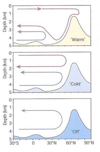
Due to large volume and thermal inertia, it is likely the deep ocean is likely (Rahmstorf, 2002). There is however, an additional complexity; the notion of thresholds in north-atlantic deepwater system. Based on Greenland and the Iberian margin, Rahmstorf (2002) shows there are 3 modes; stadial, interstadial and Heinrich mode (Figure 2). In the interstadial mode (warm, modern and interglacial), North Atlantic Deep Water (NADW) forms in the Nordic seas. In the stadial mode; it forms in the subpolar open North Atlantic (leading to a cold, glacial D-O stadial) and in the Heinrich mode, NADW formation all but ceased and waters of Antarctic origin filled deep Atlantic basin.

Figure 2: Schematic version of the three modes (‘warm’, ‘cold’ and ‘off’) of ocean circulation as observed during different times of the last glacial period. Shown is the section along the Atlantic, with NADW highlighted by the red line and AABW by the blue line.

Source: Rahmstorf (2002).

There is an enormous difficulty in quantifying the risk of abrupt changes in deep-water circulation. This is due to the possibility of a NADW bifurcation, coupled with the fact that we do not know the state of the current climate system with regards to the threshold (a point I made all the way back in post 2).

These 3 modes of deep water circulation and the bipolar seesaw mechanism highlight the non-linearity and uncertainty in our understanding of millennial-scale climate variability. This in turn, has significant implications when trying to understand and predict the impacts of climate change.